k8ik-stm/Calculations/rendered/Tunneling-Current-Distance.md

import matplotlib.pyplot as plt
import numpy as np
from pint import UnitRegistry

# Set up unit system
unit = UnitRegistry()
unit.formatter.default_format = "~"
unit.setup_matplotlib()

# Physical constants
e=-1.602176634e-19 * unit.C # electron charge
m=9.109e-31 * unit.kg # electron mass
hbar=6.62607015e-34/2/np.pi * unit.joule * unit.second # Planck constant
phi=4 * unit.eV # Work function (see table)
phi_joule=phi.to("joule")
U=5 *unit.V

# Table working functions different metals

# Metal F(eV)
# (Work Function)
# Ag (silver) 4.26
# Al (aluminum) 4.28
# Au (gold) 5.1
# Cs (cesium) 2.14
# Cu (copper) 4.65
# Li (lithium) 2.9
# Pb (lead) 4.25
# Sn (tin) 4.42
# Chromium 4.6
# Molybdenum 4.37
# Stainless Steel 4.4
# Gold 4.8
# Tungsten 4.5
# Copper 4.5
# Nickel 4.6

# Distance range
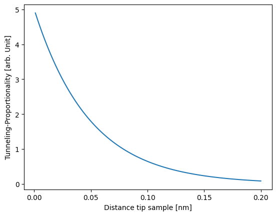
Distance_tip_sample=np.linspace(10e-13,2e-10,100)* unit.m
Tunneling_current=U*np.exp(-2*np.sqrt(2*m*phi_joule)/hbar*Distance_tip_sample) /unit.V #please note: This is not the tunneling current as this formular gives just the proportionality. Calculating the current constant is difficult as there are for us unknown parameters
Distance_tip_sample_nm=Distance_tip_sample.to("nm")

plt.plot(Distance_tip_sample_nm, Tunneling_current)
plt.xlabel(f"Distance tip sample [{Distance_tip_sample_nm.units:~P}]")
plt.ylabel(f"Tunneling-Proportionality [arb. Unit]")
plt.xticks(ticks=np.linspace(0, 0.2, 5), labels=[f"{x:.2f}" for x in np.linspace(0, 0.2, 5)])
#plt.yscale("log")

([<matplotlib.axis.XTick at 0x7e10b04929b0>,
  <matplotlib.axis.XTick at 0x7e10b04b0310>,
  <matplotlib.axis.XTick at 0x7e10b034ba60>,
  <matplotlib.axis.XTick at 0x7e10b0328670>,
  <matplotlib.axis.XTick at 0x7e10b0329360>],
 [Text(0.0, 0, '0.00'),
  Text(0.05, 0, '0.05'),
  Text(0.1, 0, '0.10'),
  Text(0.15000000000000002, 0, '0.15'),
  Text(0.2, 0, '0.20')])